The motivation to write this piece came from the FastAI course, chapter 7 on collaborative filtering. I have used embeddings in the past and understood their context in the NLP world and the relevance but in the lecture Jeremy takes you under the hood and explains what an embedding layer is. It was an aha! moment for me and motivated me to go back to some old codes that I had saved and run them again.
In image processing tasks, we have images and images have RGB channels which quantify the redness, greenness,and the blueness of the image and that can be fed to a neural net or any other machine learning algorithm to learn about the image.
But there are problems that deal with the categorical data such as:
- written text in which the relationship and context among the words isn't provided to us, or
- recommendation systems in which the relationship between the users and products isn't available to us in any usable format.
The relationship could be user from a particular age cohort, geography, or sex liking a particular product; or it could be words that are said in a particualr context such as "Coffee is as good as water" would have a differnt connotation in an airline review space vs a health magazine space.
How can we determine these relationships and contexts, so the ML models can use them? The answer is, we don't. We let the ML models learn them.
- The method is straight forward, we assign random values for let's say users and products(it can be either a single float value or a vector of values for each of the user and the product), we call these random values as latent factors.
- With some mathematical calculation, most likely a dot product, we find the approximate interaction between the user and product.
- We compare this approximate interacion with the "interaction values" such as ratings, time spent, money spent, or any other relevant metric, and find how far off our approximations are.
- We use Stochastic Gradient Descent to find the gradients and update the values that we had randomly assigned in the step 1 and repeat steps 2, 3, and 4
These upadted values or vectors of certain length are the embeddings. They encode in them the intrinsic realtionship between various factors and the context for your particular problem at hand
In the beginning, those random values didn't mean anything as they were chosen randomly, but by the end of the traning, they do as they learn on the existing data about the hidden relationships.
This YouTube video has more information, especially the part from 1:18:30 to 1:20:10
To calculate the result/interaction for a particular product and user combination, we have to look up the index of the product in our product latent factor matrix and the index of the user in our user latent factor matrix; then we can do our dot product between the two latent factor vectors. But look up in an index is not an operation deep learning models know how to do. They know how to do matrix products, and activation functions but not look ups.
We can represent look up in an index as a matrix product. The trick is to replace our indices with one-hot-encoded vectors e.g. for index 2 in a length 5 vector, the encoded vector would be
[0, 1, 0, 0, 0]
This multiplication with one-hot-encoded vectors is fine if it is done for only a few indices but for practical purposes creating too many enncoded vectors will cause memory management issues.
Most deep learning libraries avoid this problem by including a special layer that does this task of look up - they index into a vector using an intger. Also, the gradient calculated in such a manner that it is same as matrix multiplication with a one-hot-encoded vector.
This layer is called Embedding.

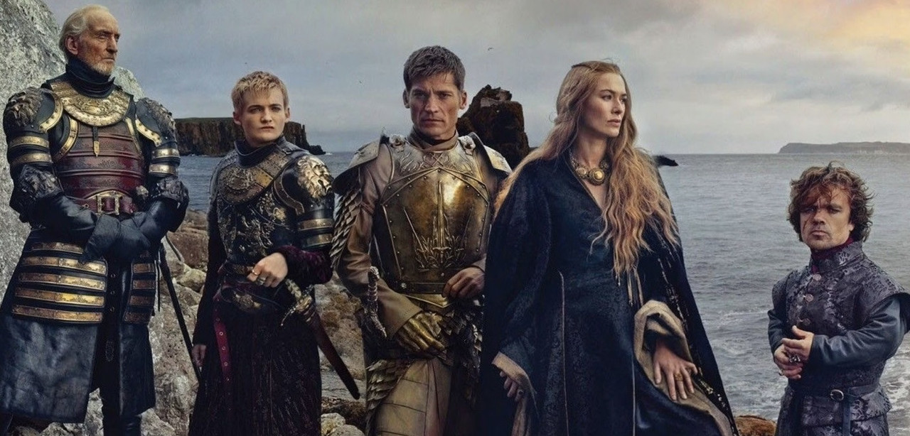
Data is present on Kaggle here, it's a text format of the five books of famous Game of Thrones
!pip install gensim
!pip install nltk
import glob
import codecs
import nltk
from nltk.corpus import stopwords
import re
import multiprocessing


import gensim.models.word2vec as w2v
import sklearn.manifold
import pandas as pd
path = "../input/game-of-thrones-book-files/"
book_filenames = sorted(glob.glob(path + "*.txt"))
print("Found books:")
for file in book_filenames:
    print(file[36:])
corpus_raw = u""
for book_filename in book_filenames:
    print("Reading '{0}'...".format(book_filename))
    with codecs.open(book_filename, "r", "utf-8") as book_file:
        corpus_raw += book_file.read()
    print("Corpus is now {0} characters long".format(len(corpus_raw)))
    print()
tokenizer = nltk.data.load('tokenizers/punkt/english.pickle')
nltk.download("punkt")
nltk.download("stopwords")
raw_sentences = tokenizer.tokenize(corpus_raw)
raw_sentences = []

with open(r'../input/sentences-corpus/sentences.txt', 'r') as fp:
    for line in fp:
        x = line[:-1]
        raw_sentences.append(x)
len(raw_sentences)
def sentence_to_wordlist(raw):
    clean = re.sub("[^a-zA-Z]"," ", raw)
    words = clean.split()
    return words
stop_words = set(stopwords.words('english'))
filtered_sentences = []
for raw_sentence in raw_sentences:
    if len(raw_sentence) > 0:
        a = sentence_to_wordlist(raw_sentence)
        filtered_sentences.append([w for w in a if not w.lower() in stop_words])
len(filtered_sentences)
c = 0
for x in filtered_sentences:
    c = c + len(x)

print("The filtered corpus contains {0:,} tokens".format(c))
num_workers = multiprocessing.cpu_count() # Fror multi threading
downsampling = 1e-3 # For frequently occurring words, downsample rate, so they don't overbeer the vocab
seed = 42 # For replication of the results
wordVectors = w2v.Word2Vec(
    sg=1, # 1 for Skip gram, 0 for CBOW
    seed=seed,
    workers=num_workers,
    vector_size=300, # How many embeddings we want per word( can be any number)
    min_count=5, # The minimum number of occurences for the word to be considered in building the word vector
    window=7, # How many neighbours of the word need to be taken into account, for the context
    sample=downsampling
)
wordVectors.build_vocab(filtered_sentences)
len(wordVectors.wv)
wordVectors.train(filtered_sentences, total_words= len(wordVectors.wv), epochs= 15)
wordVectors.wv.vectors.shape
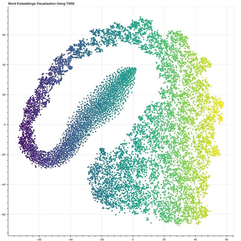
tsne = sklearn.manifold.TSNE(n_components=2, random_state=0)
all_word_vectors_matrix = wordVectors.wv.vectors
all_word_vectors_matrix
all_word_vectors_matrix_2d = tsne.fit_transform(all_word_vectors_matrix)
all_word_vectors_matrix_2d
df = pd.DataFrame(
    [
        (word, coords[0], coords[1])
        for word, coords in [
            (word, all_word_vectors_matrix_2d[wordVectors.wv.key_to_index[word]])
            for word in wordVectors.wv.index_to_key
        ]
    ],
    columns=["word", "x", "y"]
)
df.head(5)
from bokeh.plotting import figure, output_file, show, output_notebook
from bokeh.palettes import Category20
from bokeh.models import ColumnDataSource, Range1d, LabelSet, Label, CustomJS, Div, Button
from bokeh.layouts import column, row, widgetbox
from bokeh.models.widgets import Toggle
from bokeh import events
from bokeh.palettes import Spectral6
output_notebook()
from bokeh.transform import linear_cmap
from bokeh.transform import log_cmap

# create a colour map
#colourmap = {}
#for idx, cat in enumerate(categories): colourmap[cat] = Category20[len(categories)][idx]
#colors = [colourmap[x] for x in points['word']]


# create data source

source = ColumnDataSource(data=dict(
    x=df['x'],
    y=df['y'],
    name=df['word']

))

TOOLTIPS = [
    ("word", "@name"),
]


output_notebook()
#output_file(filename="TSNE.html", title="Word Embeddings Game of Thrones")


# create a new plot
p = figure(
   tools="pan,box_zoom,reset,save",
   title="Word Embeddings Visualisation Using TSNE",
   tooltips=TOOLTIPS,
   plot_width=1000, plot_height=1000
)

mapper = linear_cmap(field_name='x', palette="Viridis256" ,low=-80 ,high=60)

# add some renderers
p.circle('x', 'y', source=source, line_color=mapper, color=mapper)

labels = LabelSet(x='x', y='y', text='name', level='underlay',
              x_offset=5, y_offset=5, source=source, render_mode='canvas', text_font_size="8pt")

#p.add_layout(labels)

# show the results
show(p)
df[df["word"] == "Jon"]
wordVectors.wv.most_similar("Stark")
wordVectors.wv.most_similar("Jon")
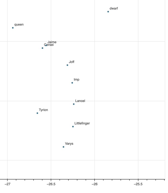
wordVectors.wv.most_similar("Tyrion")
wordVectors.wv.most_similar("Cersei")
alt.data_transformers.disable_max_rows()
import altair as alt

source = df

alt.Chart(source).mark_circle(size=60).encode(
    x='x',
    y='y',
    tooltip=['word']
).properties(
    width=900,
    height=800
).interactive()